A classification of natural rivers
Original study by Rosgen, D. L. in CATENA 22 (3):169–199. https://linkinghub.elsevier.com/retrieve/pii/0341816294900019.
and Replication by: Kasprak, A., N. Hough-Snee, T. Beechie, N. Bouwes, G. Brierley, R. Camp, K. Fryirs, H. Imaki, M. Jensen, G. O’Brien, D. Rosgen, and J. Wheaton. 2016. The Blurred Line between Form and Process: A Comparison of Stream Channel Classification Frameworks ed. J. A. Jones. PLOS ONE 11 (3):e0150293. https://dx.plos.org/10.1371/journal.pone.0150293.
Replication Authors: W. Steven Montilla M., Zach Hilgendorf, Joseph Holler, and Peter Kedron.
Replication Materials Available at: Rosgen repository
Created: 24 March 2021
Revised: 9 April 2021
Introduction
The classification of rivers and streams is important to understand their diversity and distribution (Kasprak et al. 2016). General characterizations of fluvial bodies can serve as an important tool to develop conservation, management and restorations plans (Kasprak et al. 2016). However, developing a classification schema for rivers and streams is a hard task. The everchanging nature of these systems as well as the practicality to take measurements on the field are limitations to river classification. The various classifications methods available may also produce different results on the same river. Therefore, Kasprak et al. (2016) were motivated to conduct a direct comparison between 4 different classification frameworks to analyze their agreements and discrepancies.
Kasprak et al (2016) conducted their study in the Middle Fork John Day Basin within the Columbia River Basin in Oregon, USA. They classified rivers/ streams on 33 sites using the River Styles Framework, Natural Channel Classification, Rosgen Classification System, and a channel form-based statistical classification.
As a class, we replicated the Rosgen classification portion of the Kasprak et al (2016) study. Each student was assigned one of the 33 sites to carry out the replication of the Rosgen classification. I was assigned Loc_ID 8, Granite Boulder Creek.
Data
ALL DATA/ Metadata CAN BE FOUND HERE
- Camp Creek Lidar DEM data: This is the John Day River watershed LiDAR DEM. The LiDAR dataset is a 1 m resolution bare earth DEM that was collected between Aug 19-27, 2008. The dataset was larger, but was clipped down for the purposes of easily sharing data. The main focus of the raster is the Middle Fork of the John Day River and encompasses all CHaMP data provided in the CHaMP_Data_MFJD dataset.
LiDAR data and the associated metadata were downloaded from the Oregon Department of Geology and Mineral Industries (DOGAMI) data portal at https://gis.dogami.oregon.gov/maps/lidarviewer/.
- CHaMP_Data_MFJD The Columbia Habitat Monitoring Program (CHaMP) observed 26 watersheds in the Columbia River watershed, chosen to maximize contrasts in current habitat conditions. The main goal of this monitoring program was to generate and implement a set of standard methods for monitoring fish habitat (https://www.champmonitoring.org/). The Kasprak et al. (2016) article employed a variety of classification schemes using the CHaMP dataset, including the Rosgen Stream Classification method. The data provided for this module is a subset of the overall dataset, that overlapped with available bare earth light detection and ranging (LiDAR) digital elevation models (DEM) for the state of Oregon, USA. The subset includes points within the Middle Fork John Day River (MFJD).
Methods
Original Study Information
- The Kasprak et al. (2016) paper can be found here
Kasprak et al. (2016) followed the Rosgen Classification System (RCS) on Level I and II (Fig. 1) to generate the classifications. They used DEMs (0.1m grid resolution), aerial imagery (1m res), and ground-based assessments to calculate the ratios needed in Level I. In their case, they used the used the River Bathymetry (RBT) to calculate width to depth and entrenchment and sinuosity. Moreover, they processed elevation models using the CHaMP Topo Toolbar. They relied on the CHaMP surveys to inform median grain size (D50) at each point and classify each reach to Level II in the RCS.
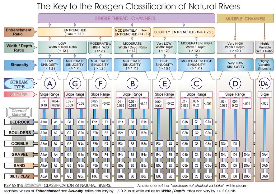 Figure 1. Rosgen Classification System.
Replication
Each student in our class was randomly assigned one of the 33 CHaMP points to replicate the RCS classification. I was assigned Loc_ID 8, Granite Boulder Creek.
- CHaMP sites at the Middle Fork John Day Basin: My assigned site is highlighted in blue. -You can see different information collected by the CHaMP surveys by clicking on a site of interest. -This layer can be found on the data repository linked above. CHaMP sites
Processing of Raster Data
Step by step protocols can be found here
Raster Lidar data was processed using this model to visualize elevation (Fig. 3) and Percent slope (Fig. 4) following the workflow seen in Fig 2. Note that the rasters were reclassified and colorized in QGIS to provide more contrast within the study site. This model also produces a buffer with a radius of 20 channel widths, which will serve as our area of interest.
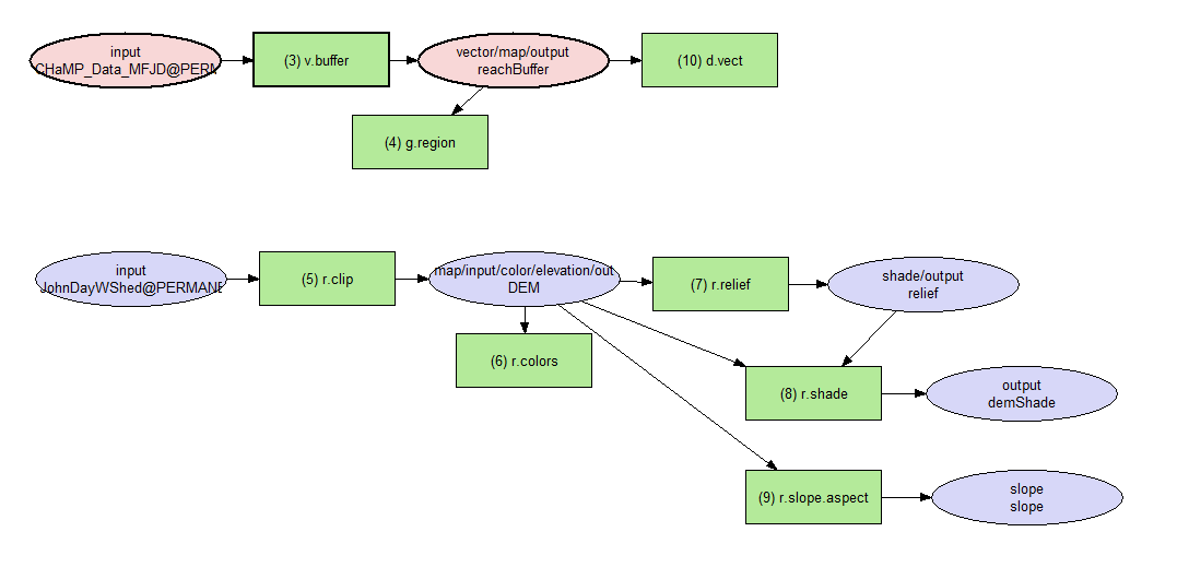 Fig 2. Visualization workflow
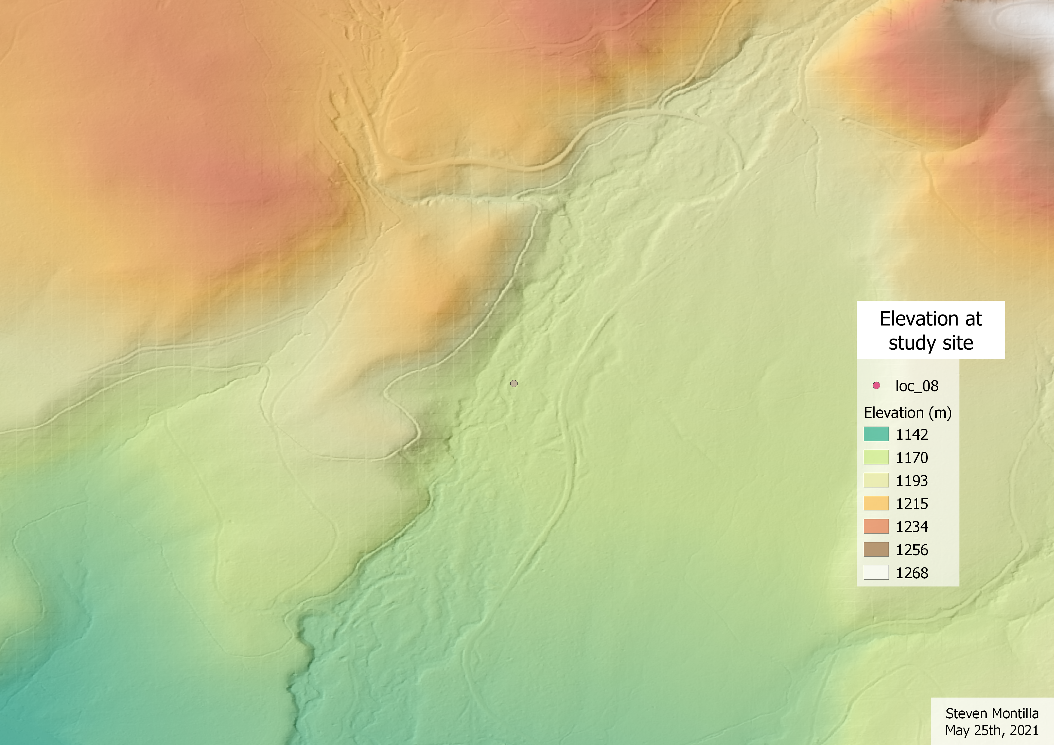 Fig 3. Shaded elevation model
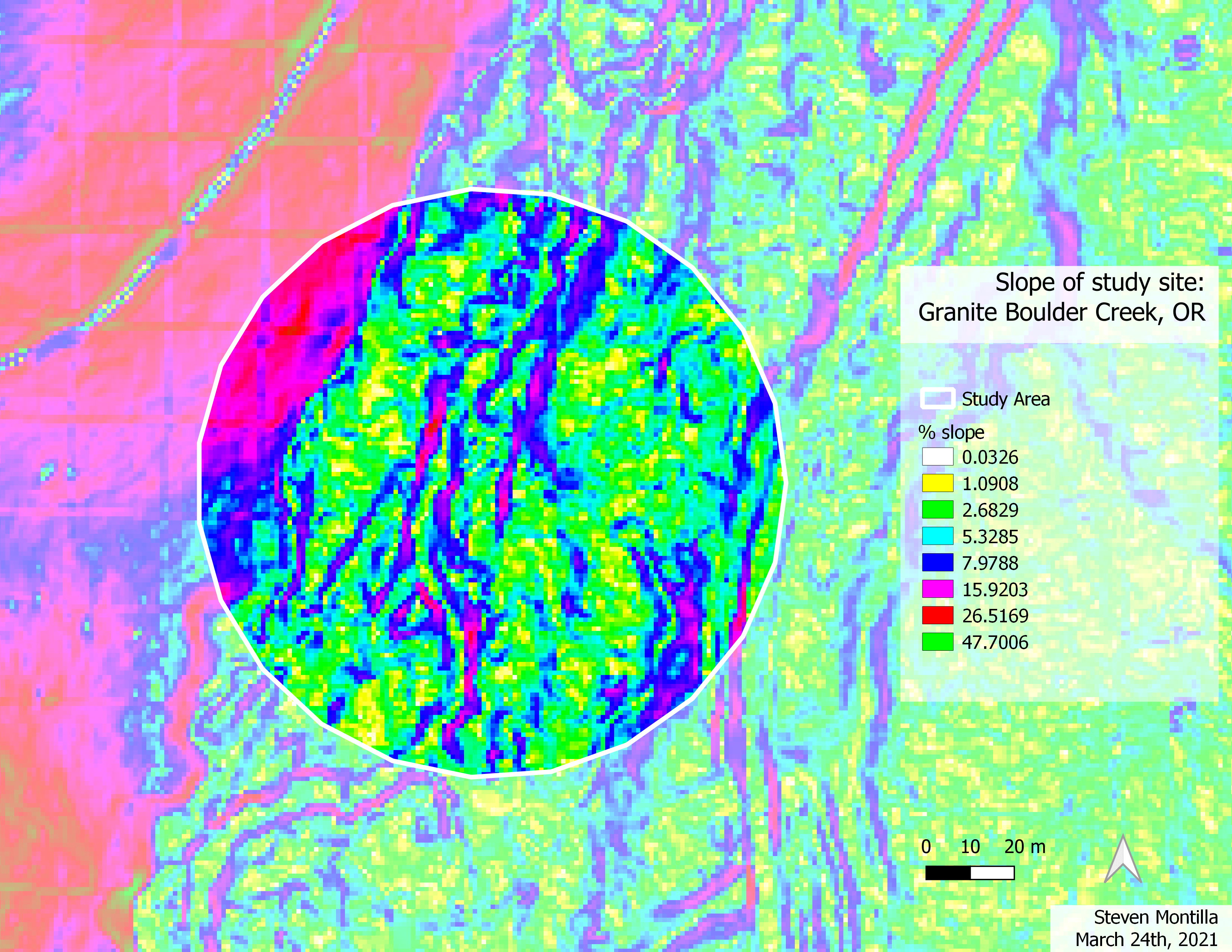 Fig 4. Percent slope model
Digitizing of River Banks and Valley width
I digitized the bankfull channel and valley channel using the elevation and slope models at a scale of 1:1500. This process was done three times, alternating between digitizing the bank and the valley to reduce the impact of muscle memory. Centerlines were calculated from each set of channel lines, which then were averaged into a mean stream bank centerline (Fig. 5) and a mean valley centerline (Fig. 6) using this model.
Troubles digitizing
In my case, I re-digitized the channels after noticing that my digitization was well off the real course of the river. I used Google Earth Pro to look at imagery from 2007 (the closest to the date of data collection of CHaMP data - 2012). The second digitization yielded more similar results to the Kasprak et al.(2016) classification. Nevertheless, looking back at my work, I did not have the correct map for elevation while I was digitizing, which made it harder and more confusing to do. When I fixed the elevation map, the river channels became much more apparent than what I was seeing in the first map I made. However, I was not able to re-digitize the river due to time constraints. However, I will be more attentive to having the correct elevation and slope models before starting digitization in the future.
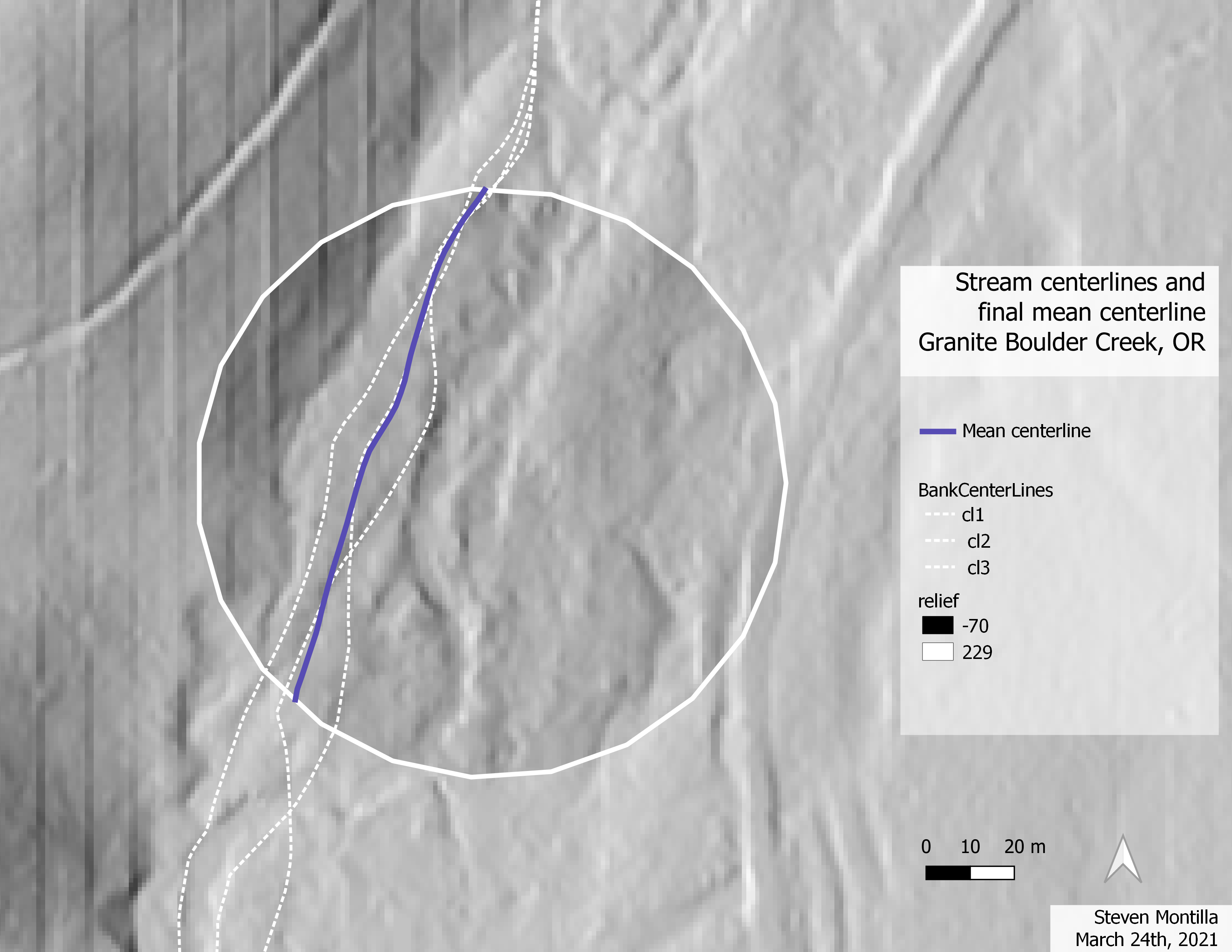 Fig 5. Stream centerline average and uncertainty
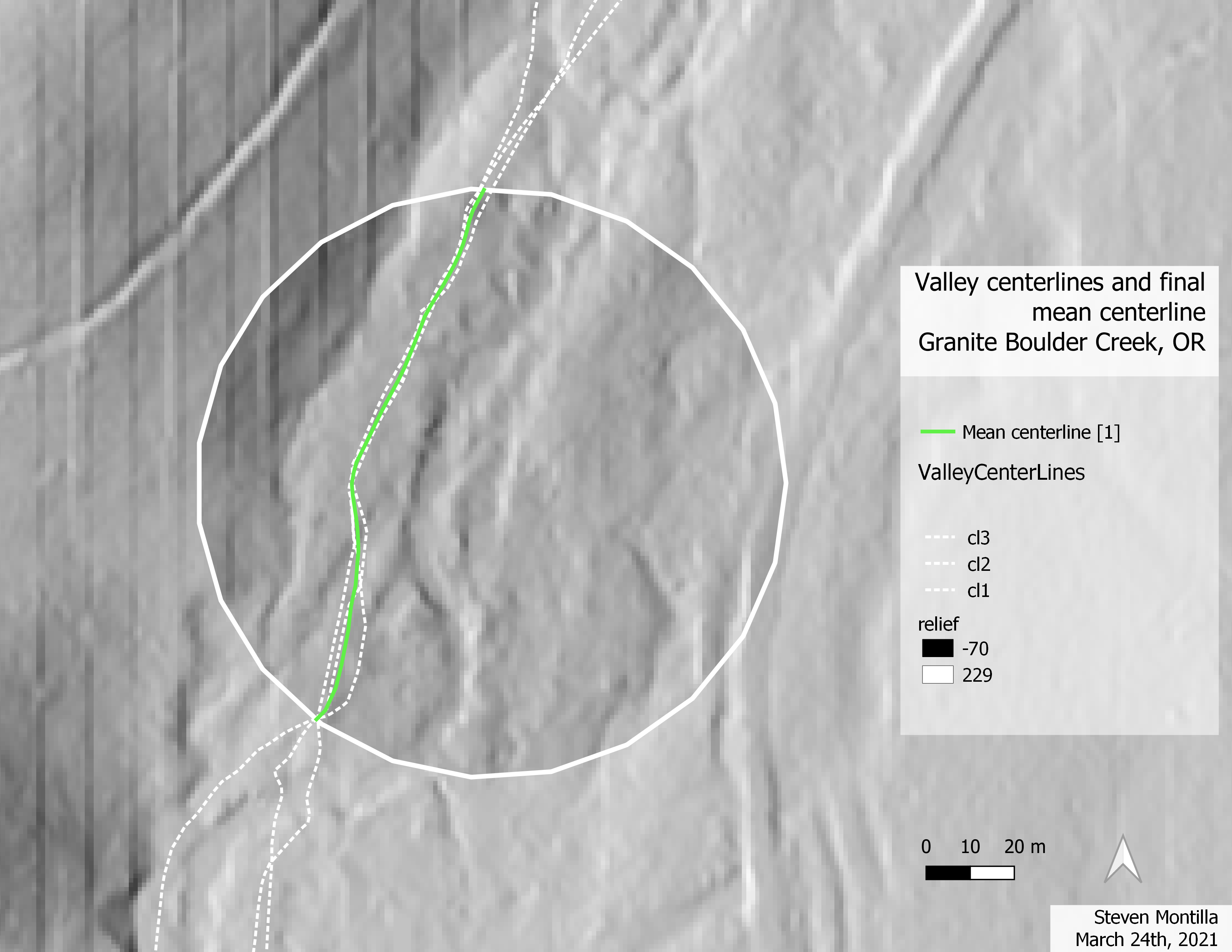
Fig 6. Valley centerline average and uncertainty
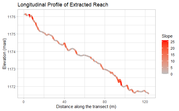
Fig 7. Longitudinal Profile
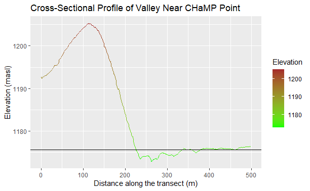
Figure 8. cross-sectional profile of Valley near CHaMP Loc_ID 08
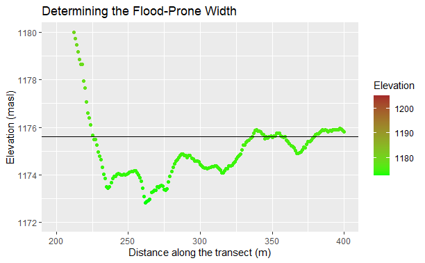
Figure 8. cross-sectional profile of banks near CHaMP Loc_ID 08
Calculation on ratios
According to the Rosgen classification schema, in order to classify a stream you need the entrenchment ratio, width to depth ration and the sinuosity. The following table summarizes where the data to calculate these ratios came from.
Table 1. Site Measurements
| Variable | Value | Source |
|---|---|---|
| Bankfull Width | 5.932 | CHAMPS attribute table |
| Bankfull Depth (mean) | 0.2426 | CHAMPS attribute table |
| Bankfull Depth (max) | 1.0406 | CHAMPS attribute table |
| Valley Width | 105 | crossectional profile |
| Valley Depth | 2.0812 | 2 * bankfull depth (max) |
| Stream/River Length | 124.217654 | banksLine attribute table |
| Valley Length | 128.759278 | valleyLine attribute table |
| Median Channel Material Particle Diameter | 67 | CHAMPS attribute table |
Results
The following tables and figure summarize the results. Essentially, the Granite Boulder Creek was classified as stream type C4b
Table 2. Rosgen Level I Classification
| Criteria | Value |
|---|---|
| Entrenchment Ratio | 17.70060688 |
| Width / Depth Ratio | 24.45177246 |
| Sinuosity | 1.164727792 |
| Level I Stream Type | C |
Table 3. Rosgen Level II Classification
| Criteria | Value |
|:——————–:|:——-:|
| Slope | 0.03205 |
| Channel Material | Gravel |
| Level II Stream Type | C4b |
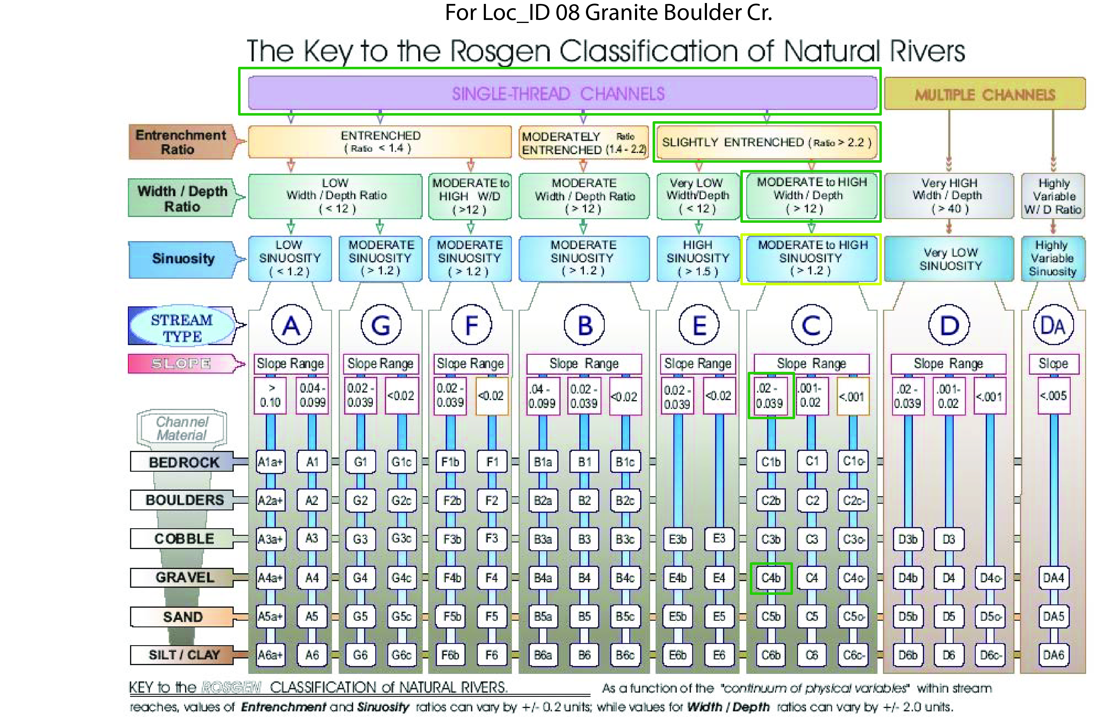
Fig.6 Rosgen schema with highlighted categories.
Discussion
The Boulder Granite Creek at this site was classified as a C4b stream which is in agreement to Kasprak’s classification (Kasprak et al, 2016). As seen in Table 2 and Figure 6, all the entrenchment and width to depth ratios fell within the ranges established by the Rosgen key. I calculated a sinuosity value of 1.16 that fell short of the > 1.2 required for the C stream type. However, for the sinuosity value, the Rosgen classification specifies that entrenchment and sinuosity can be within a +/- 0.2 error margin. Taking this margin into account would bring my sinuosity value to 1.18 which could be rounded to 1.2, marginally less than the > 1.2 required to be classified as a stream type C. I decided to still go through with classifying this stream as type C because the small margin could be accounted for by errors in digitization that could result in lower sinuosity values. Specifically, it was difficult to know exactly the course of the stream using the elevation model which could have lead to an oversimplification of the curvature of the stream, resulting in lower sinuosity values. Moreover, the Rosgen key does not provide any alternatives for a sinuosity lower than 1.2 with the values for width to depth and entrenchment ratios shown in table 2.
For the Level II classification, the percent slope was within the range established. Moreover, we were not able to collect our own channel material data, so we used the one registered by the CHaMP.
Conclusions
This replication was successful at obtaining the same results as Kasprak et al. (2016) did for this study site using the Rosgen classification key. Nonetheless, there would be more confidence in the methods and results that were obtained by having first hand field observations. As mentioned above, the digitization of the bank and valley was done without much context of the site, depending only on elevation models that were personally challenging to interpret. Since this was a replication study, there was more confidence on the results obtained because they could be compared to Kasprak et al (2016). However, if this study had not had a comparison point, I would have not been confident that the results were accurate, since we lacked more field observations and experience digitizing waterways from elevation models.
Finally, there is great potential in relying on lidar elevation data and this methodology to classify rivers and streams. Undoubtedly, this would be more efficient than visiting each site and conducting the classification ‘by hand’. Nonetheless, I do think that the analysts doing this kind of work should have more experience deducing river banks and valleys accurately from elevation models to increase the confidence in the results of the methodology.