RP- Vulnerability modeling for sub-Saharan Africa

Replication of

Vulnerability modeling for sub-Saharan Africa

Original study by Malcomb, D. W., E. A. Weaver, and A. R. Krakowka. 2014. Vulnerability modeling for sub-Saharan Africa: An operationalized approach in Malawi. Applied Geography 48:17–30. DOI:10.1016/j.apgeog.2014.01.004

Replication Authors: W. Steven Montilla M., Joseph Holler, Kufre Udoh, Open Source GIScience students of fall 2019 and Spring 2021

Replication Materials Available at: RP-Malcomb forked repository

Created: 25 April 2021 Revised: 27 April 2021

Abstract

The original study is a multi-criteria analysis of vulnerability to Climate Change in Malawi, and is one of the earliest sub-national geographic models of climate change vulnerability for an African country. The study aims to be replicable, and had 40 citations in Google Scholar as of April 8, 2021.

Original Study Information

The study region is the country of Malawi. The spatial support of input data includes DHS survey points, Traditional Authority boundaries, and raster grids of flood risk (0.833 degree resolution) and drought exposure (0.416 degree resolution).

The original study was published without data or code, but has detailed narrative description of the methodology. The methods used are feasible for undergraduate students to implement following completion of one introductory GIS course. The study states that its data is available for replication in 23 African countries.

Data Description and Variables

Outline the data used in the study, including:

• sources of each data layer and
• the variable(s) used from each data source
• transformations applied to the variables (e.g. rescaling variables, calculating derived variables, aggregating to different geographic units, etc.)

Overview

Malcomb et al. (2014) calculated household resilience seen in scores using three different data sources (refer to Fig. 2 of Malcomb et al. 2014)

• The variables to calculate Adaptive Capacity were obtained from the USAID’s Demographic and Health Surveys (DHS).
• Livelihood sensitivity variables were taken from the USAID’s Famine Early Warning Systems Network (FEWSNET).
• Finally, physical exposure variables were taken from the United Nations Environment Programme (UNEP).

Background of Data Sources

USAID’s Demographic and Health Surveys

Demographic and Health Surveys (DHS) are nationally-representative household surveys that provide data for a wide range of monitoring and impact evaluation indicators in the areas of population, health, and nutrition (from DHS website). These surveys record assets and access to resources at the household level. The following list outlines the specific variables that were taken into account in this part of the replication. Specifically, DHS data was only used to obtain assets and access data to calculate Adaptive Capacity (40% of the Household Resilience Score). DHS data requires use authorization by the DHS and therefore cannot be shared in this report or through the data repository. You can get authorization to obtain the data on this here
For ASSETS

Name listed by Malcomb et al. (2014)	Variable (from DHS 2010) used in replication	Possible values
# Livestock Units (4%)	Livestock, herds or farm animals	yes or no
	NA - cows, bulls own	0 - 95+, unknown
	NA - horses, donkeys, mules own	0 - 95+, unknown
	Goats own	0 - 95+, unknown
	Sheep own	0 - 95+, unknown
	Poultry own	0 - 95+, unknown
	Other own	0 - 95+, unknown
Arable Land (Hectares) (6%)	“Hectares for agricultural land”	95 or more 98 “unknown”
# in Household Sick in Past 12 mo (3%)	“Member has been very sick for 3+ months last year”	YES/ NO/ DK
	“Mother has been very sick for 3+ months last year”	YES/ NO/ DK
	“Father has been very sick for 3+ months last year”	YES/ NO/ DK
	“Mother/father dead or been very sick for 3+ months”	YES/ NO/ DK
Wealth Index Score (4%)	DHS 2010, HV270	poorest, poorer, middle, richer, richest
# of Orphans in Household (3%)	Number of orphans and vulnerable children	n

For ACCESS

Name listed by Malcomb et al. (2014)	Variable (from DHS 2010) used in replication	Possible values
Time to water source (4%)	Time to get to water source	On premises, do not know
Electricity (3%)	Has electricity	Yes/NO
Type of cooking fuel (2%)	Type of cooking fuel	Electricity, LPG/Natural gas, Natural gas, Biogas, Kerosene, Coal/lignite, charcoal, wood, straw/shrubs/grass, agricultural c rop, animal dung, no food cooked, other
Sex of head of household (2%)	“Sex of head of household”	Male, Female
Own a cell phone (4%)	has a mobile telephone	Yes/NO
Own a radio (3%)	Has Radio	Yes/NO
House setting (urban/rural) (2%)	type of place of residence	Urban, Rural

USAID’s Famine Early Warning Network (FEWSNET)

FEWSNET, the Famine Early Warning Systems Network, is a leading provider of early warning and analysis on acute food insecurity around the world (from FEWSNET website). One of the goals of the FEWSNET is to predict future cases of acute food insecurity in order to inform humanitarian response. Therefore, the data they collect is tailored towards measuring the vulnerability of communities mainly focused on land use practices, food sourcing, and coping strategies of the communities surveyed. Malcomb et al. (2014) used variables from the FEWSNET 2005 survey in Malawi to calculate the 20% Livelihood Sensitivity portion of the Household Resilience scores. However, they were not clear on which variables exactly they used, so we had to use our judgement to make the our best informed guesses. The following table shows the attributes and calculations that we carried out in contrast to what was listed in the paper.

Name listed by Malcomb et al. (2014)	**Variable (from FEWSNET 2005) used in
replication**	Possible values
Food From Own Farm (6%)	Sources of food: crops	x%
Income From Wage Labor (6%)	Sources of Cash: labour / total income	x%
Income From Cash Crops (4%) (% labor that is susceptible to market shocks (tobacco, sugar, tea, coffee))	Sources of cash: crops / total income (Included income from all crops due to vague definition of cash crops)	x%
Disaster Coping Strategy (4%) (potential sources of additional food and income that lead to environmental degradation)	Income from sales of firewood, grass, wild foods / total income	x%

United Nations Environment Programme (UNEP)/ Global Resource Information Database (GRID) Data:

The GRID-Geneva database comes from a partnership between the UNEP, the Swiss Federal Office for the Environment and the University of Geneva. Their focus is on processing, analysis and creating models from satellite data using remote sensing techniques and GIS with the goal of providing scientific information to decision makers.(Learn more here) The Global Risk Data Platforms is the product of a multiagency effort to share spatial information on global risk from natural hazards. (Learn more here)

• Following the procedure from Malcomb et al. (2014), we obtained the Estimated Risk for Flood Hazard and Exposition to Drought Events layers from this data source.

Data transformations

The first transformation of the data was normalization. Since all variables used came in different units, it would be impossible to compare them without normalizing them. Malcomb et al. (2014) do so by transforming all variables to a scale of 0-5 (6 data categories). However, the script becomes confusing when they mention that they used quintiles (5 data categories). Since their highest score was 5, but they only had 5 categories, we used the quintile breaks and modified it to be a scale from 1-5 resulting in 5 total categories.

Capacity scores were weighted following table 2. of Malcomb et al. and then summed to calculate capacity scores with the corresponding weighted variables. We multiplied the score by 20 to match the scale on Malcomb et al’s figures.

Analytical Specification

The original study was conducted using ArcGIS and STATA, but does not state which versions of these software were used. The replication study will use R.

Materials and Procedure

Workflow First Version

1. Step 1: Preprocessing of Geographic Boundaries

DHS Households table (1 row/house) → field calc → conversion to 0-5 scale → weighted A/C score → join by attribute w/ DHS data points (village level) → spatial join AND group w/ traditional authorities (GADM adm_2) → traditional authorities w/ Capacity Score → Raster

Drought exposure → rescale 0-5

Flood risk → rescale 0-5

Livelihood zones → copy #s from spreadsheet →rescale 0-5 → Rasterize → Raster Calc (w/ Drought Exposure and Flood Risk Rasters)

1. Step 2 Data Input: UNEP/grid Europe, Famine early warning network → Raster → Weight values: All vulnerability measures were weighted (table 2) and normalized between 0 & 5 (RStudio)

2. Step 3: Creating the Model of Vulnerability Calculate: Household resilience = adaptive capacity + livelihood sensitivity - biophysical exposure

Revised Version

1. Download traditional authorities: MWI_adm2.shp
2. Adding TA and LZ ids to DHS clusters
3. Removing HH entries with invalid or unknown values
4. Aggregating HH data to DHA clusters, and then joining to traditional authorities to get: ta_capacity_2010
5. Removing index and livestock values that were NA
6. Sum of Livestock by HH
7. Scale adaptive capacity fields (from DHS data) on scale of 1 - 5 to match Malcomb et al.
8. Weight capacity based on table 2 in Malcomb et al.
9. Calculate capacity by summing all weighted capacity fields
10. Joining mean capacities to TA polygon layer
11. Summarize capacity from households to traditional authorities
12. Making capacity score resemble Malcomb et al’s work (scores on range of 0-20) by multiplying capacity score by 20
13. Categorizing capacities using natural jenks methods
14. Creating blank raster and setting extent of Malawi - CRS: 4326
15. Reproject, clip and resampling flood risk and drought exposure rasters to new extent and cell size
16. Uses bilinear resampling for drought to average continuous population exposure values
17. Uses nearest neighbor resampling for flood risk to preserve integer values
18. Removing factors and recasting them as integers
19. Clipping TAs with LZs to remove lake
20. Rasterizing final TA capacity layer
21. Masking flood and drought layers
22. Reclassify drought raster into quantiles
23. Add all RASTERs together to calculate final output: final = (40 - geo) * 0.40 + drought * 0.20 + flood * 0.20
24. Use zonal statistics to aggregate raster to TA geometry for final calculation of vulnerability in each traditional authority

Final version

After compiling the missing data for Livelihood Sensitivity, we integrated it to the analysis following this final version of the workflow:

1. Data Preprocessing:
2. Download traditional authorities: MWI_adm2.shp
3. Adding TA and LZ ids to DHS clusters
4. Removing HH entries with invalid or unknown values
5. Aggregating HH data to DHS clusters, and then joining to traditional authorities to get: ta_capacity_2010
6. Removing index and livestock values that were NA
7. Sum of livestock by HH
8. Scale adaptive capacity fields (from DHS data) on scale of 1 - 5 to match Malcomb et al.
9. Weight capacity based on Table 2 in Malcomb et al.
10. 1. Calculate capacity by summing all weighted capacity fields
11. Summarize capacity from households to traditional authorities
12. Joining mean capacities to TA polygon layer
13. Making capacity score resemble Malcomb et al.’s work (scores on range of 0-20) by multiplying capacity score by 20
14. Categorizing capacities using natural jenks methods
15. Creating blank raster and setting extent of Malawi - CRS: 4326
16. Reproject, clip and resampling flood risk and drought exposure rasters to new extent and cell size
    • Uses bilinear resampling for drought to average continuous population exposure values
    • Uses nearest neighbor resampling for flood risk to preserve integer values
    • Removing factors and recasting them as integers
    • Clipping TAs with LZs to remove lake
    • Rasterizing final TA capacity layer
17. Masking flood and drought layers
18. Reclassify drought raster into quantiles
19. Add all RASTERs together to calculate final output: final = (40 - geo) * 0.40 + drought * 0.20 + flood * 0.20 + livelihood sensitivity * 0.20
20. Using zonal statistics to aggregate raster to TA geometry for final calculation of vulnerability in each traditional authority

Finally, the results of the reproduction and the original study were compared using a couple of methods. To compare the choropleth adaptive capacity maps we generated a confusion matrix and calculated Spearman’s rho coefficient. For the raster vulnerability maps, we plotted the values of each cell in Figure 6. below. Perfect agreement would have resulted in alignment of all the points along the diagonal, but there was little agreement thus the messy graph and the low spearman’s rho coefficient.

Reproduction Results

The reproduction of the adaptive capacity classification had a strong similarity (rho = 0.7711839) with the original map. In the case of the vulnerability maps, we observed a Spearman’s rho coefficient = 0.2686568 showing high dissimilarity between Malcomb et al’s results and ours.

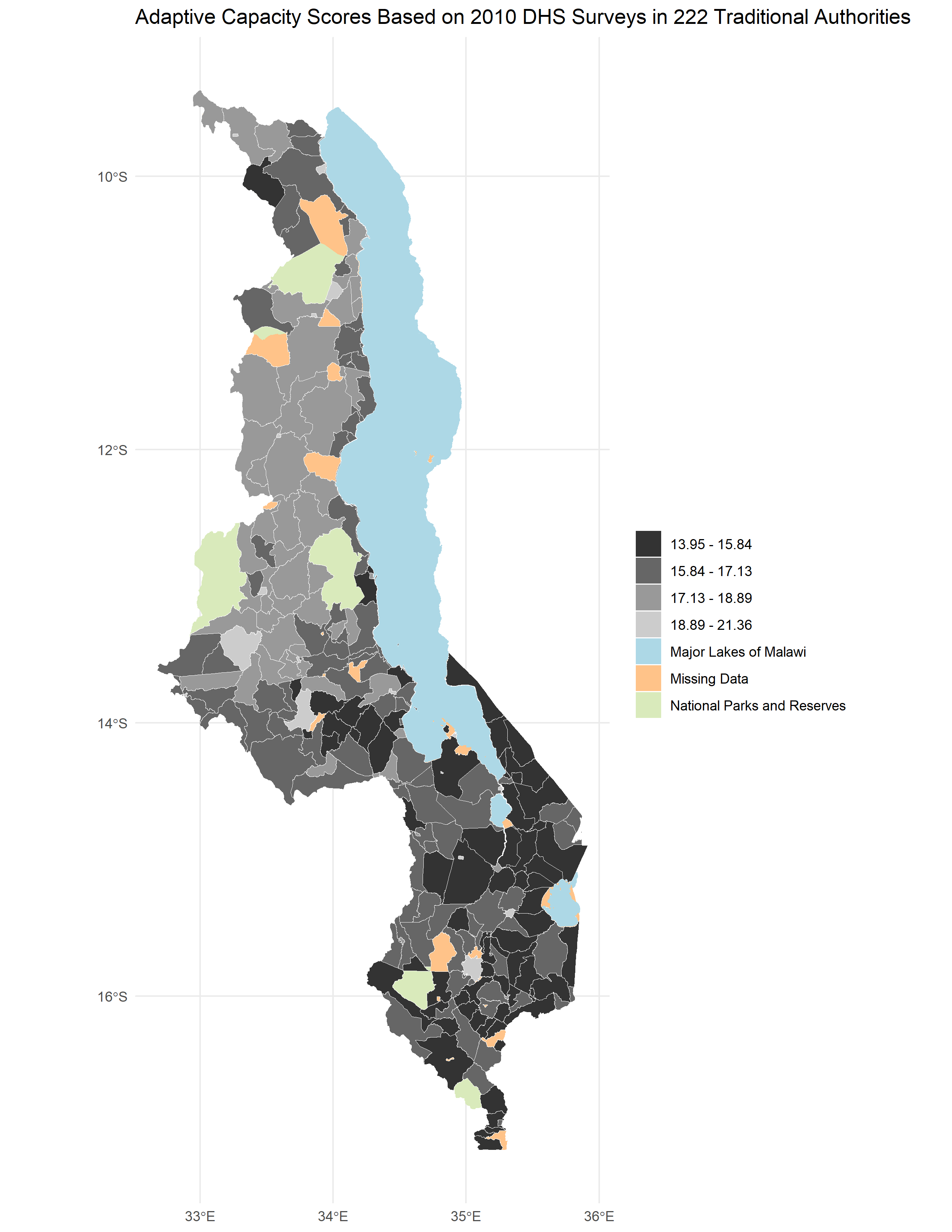
• Figure 1. Reproduced map of adaptive capacity in Malawi analogous to Malcomb et al’s figure 4.

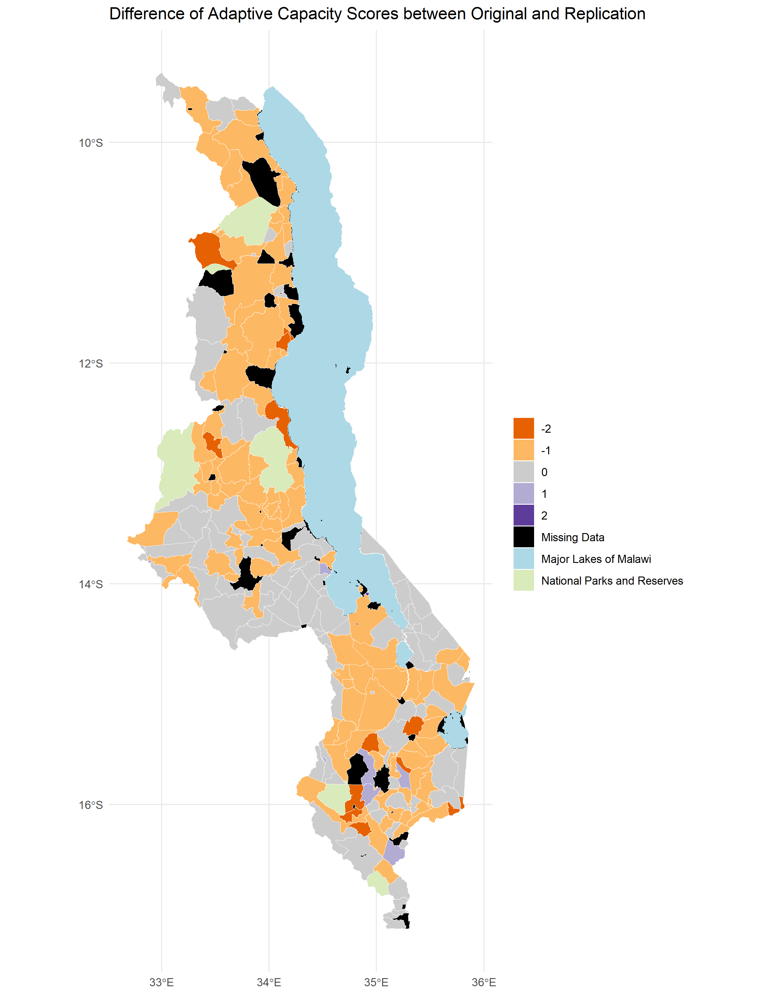
• Figure 2. Difference between reproduced adaptive capacity map and Malcomb et al’s.

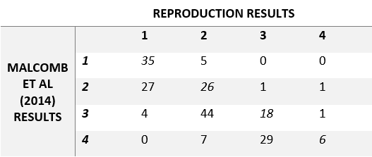
• Figure 3. Confusion matrix for Malcomb et al’s Figure 4 and our outcome.

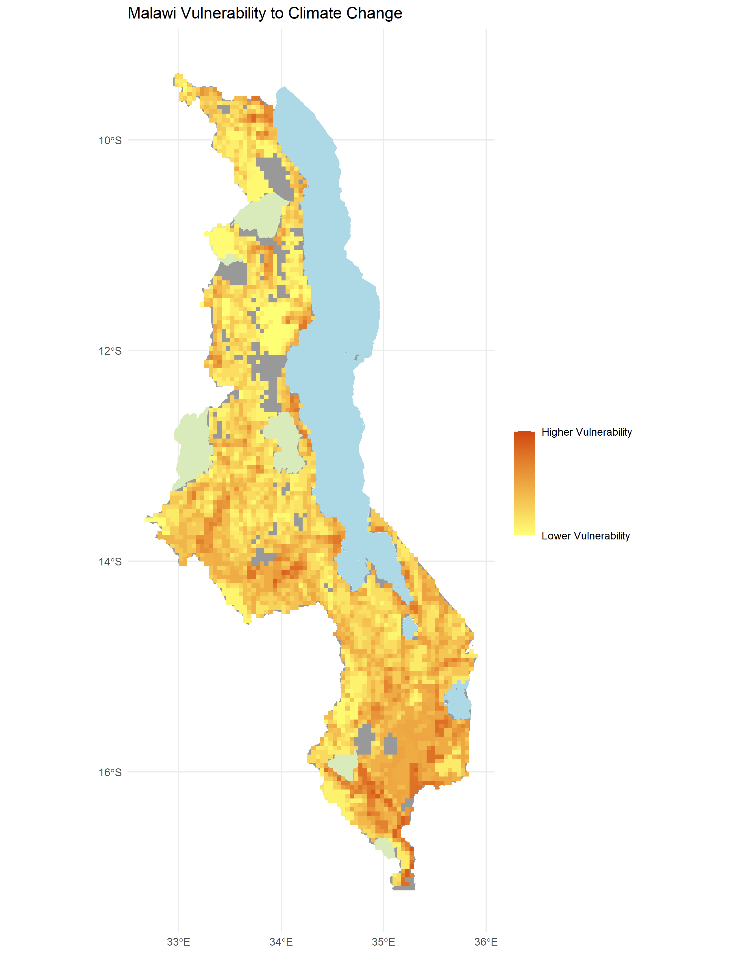
• Figure 4. Reproduced map of vulnerability in Malawi analogous to Malcomb et al’s Figure 5.

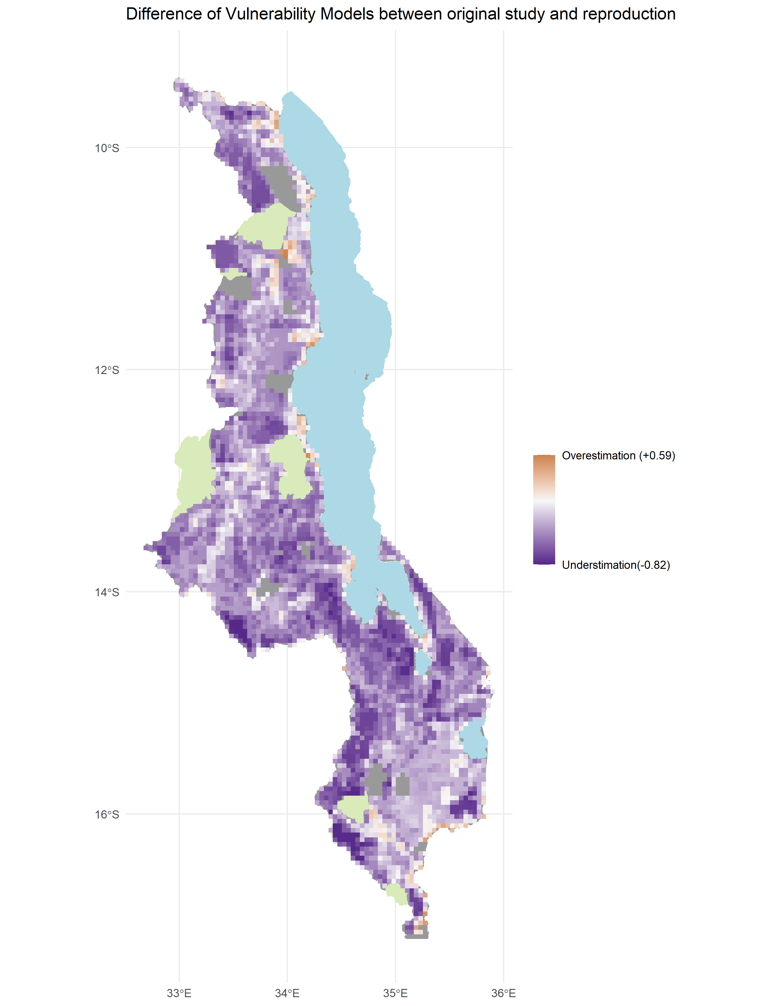
• Figure 5. Difference between reproduced vulnerability map and Malcomb et al’s.

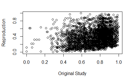
• Figure 6. Plot of similarity between the reproduced vulnerability scores and Malcomb et al’s.

Unplanned Deviations from the Protocol

• As mentioned above, at first we thought that Malcomb et al. had normalized all the variables in a 0-5 scale as they mention on the paper. However, after inspecting the article more and talking about this issue in class, we decided to normalize the data in a 1-5 scale using the quintiles Malcomb et al. confusingly also mention.
• When looking at the adaptive capacity maps from Malcomb et al., we noticed that our results were in another scale, so we decided to multiply the results by 20 to fit the scale that Malcomb et al. used in their maps. However, the true reason why the scores were modified or how they got their results in that scale is unknown to us.
• On a similar note, the Livelihood Sensitivity attributes were taken from the FEWSNET dataset pretty much arbitrarily. We did not know how Malcomb et al used that data specifically neither did we know what attributes they used. Malcomb et al. provide a list of indicators in Table 1. but the ones listed under Livelihood Sensitivity were not specifically named that in the FEWSNET dataset. To resolve this, as a group we gathered our best informed guesses and calculated values for each variable as shown in the data section above.

Discussion

This reproduction of Malcomb et al (2014) was somewhat successful. Malcomb et al. (2014) claimed their study to be very reproducible. As Prof. Holler mentioned, it has been cited a considerable amount of times in the literature. Morever, we followed Malcomb et al’s (2014) methodology to the best of our ability and used the same data. Therefore, it is dissapointing that we got such dissimilar results.

Regarding the reproduction of the adaptive capacity map, there was a high Spearman’s rho coefficient of 0.7711839 between the map our classification and the original study. However, it is worth questioning whether this is good enough for a reproduction of a study where the same data is being used. Especially considering that there was less uncertainty when getting the data for adaptive capacity than for llivelihood sensitivity. Possible explanations for the difference between the original study and our reproduction may be related to some of the deviations mentioned in the previous section. For example, our interpretation of the scaling that Malcomb et al (2014) conducted in the original study may be wrong, introducing uncertainty to our results. Similarly, the rescaling of the results by multiplying by 20 may have also introduced uncertainty given that Malcomb et al did not specifically outlined how they came up with adaptive capacity scores in that scale.

Regarding the vulnerability map reproduction, we were not as successful in reproducing Malcomb et al’s results. With a rho coefficient of 0.2686568, there was little agreement between the original study and the reproduction. As seen in figure 5. our reproduction largely underestimated vulnerability except for a few areas on the coast, which were overestimated. The disagreement between the original study and our results could be attributed to the lack of clarity in the description of the methods. We only had the limited narrrative of the methods in the paper and no code or detailed workflow to follow.

In general terms, sources of uncertainty for this replication study were present at two different levels. Firstly, regarding the original study, there was epistemic uncertainty introduced by the creation of the vulnerability index due to subjective input used to make decision in the model. As Tate(2013) states, this type of uncertainty is the result of utilizing expert opinion and community surveys in the selection of parameters and weighting of the resilience index calculated in the original study. Malcomb et al (2014) conducted interviews to identify metathemes to frame their surveys and include variables to resilience index that were meaningful in understanding vulnerability in the Malawian context. However, the kinds of questions Malcomb et al. (2014) asked in these interviews may have also skewed the topics talked about in the interviews and therefore affect the metathemes identfied through those surveys. Moreover, uncertainty can be explained through Longley et al’s (2008) conceptualization of uncertainty. In this model, there is more distortion of the way the real world is conceived as data is transported and translated in different units of analysis. In this case, the transformatio of the data into normalized indices and aggregation to different geographic scales may have also introduced uncertainty.

Finally, there was no further verification of the resilience model by Malcomb et al. (2014). Therefore, there was no clear way to know if the areas that the study deemed as more resilient or not actually were. It is important to mention that proving the veracity of these kinds of models is difficult to do pre-disaster. In other words, one of the ways to know the accuracy of a vulnerability model would be to compare its predictions to the impacts of an actual incident in the place. Clearly, if this were the case a lot of the value in coming up with vulnerability models would be undermined. The whole purpose of this kind of studies is to identify areas where disaster prevention and preparation efforts should go to. As Tate (2013) explain, a Monte Carlo simulation may be appropriate to analyze epistemic uncertainty in the model. This simulation iterates the vulnerability model changing its configuration each time. The results allow us to understand how the deliberate decision of the authors influenced the results of the model. Given that this study was made completely in R, the Monte Carlo simulation is very feasible!

Conclusion

This reproduction study was an example of how difficult it is to replicate geospatial research with current standards of publication and the shortcomings of vulnerability modeling. There are two main sources of uncertainty that play into the difficulty to replicate the study. Firstly, the epistemic uncertainty introduced by the deliberate decisions of the authors that may not be very well communicated through their writing. Secondly, the lack of a clear objective methodology to follow (i.e. workflow, code script, etc…) made it difficult to have certainty about the decisions we made about normalizing (0-5 or 1-5 scale), or choosing attributes for livelihood sensitivity. Finally, the results of this reproduction are another example of the need for higher standards of publication regarding the documentation of methods and availability of data and software to ensure that scrutiny, replicability and reproducibility of the study is possible and accurate.

Acknowledments

Thanks to Prof. Joseph for organizing this lab and preparing the materials. To Kufre Udoh for developing the reproduction script in R, helping me resolve problems with the code, and answering questions. Likewise, credit to my lab group: Arielle Landau for guiding us in understanding the code, Maddie Tango and her issues submissions for helping me troubleshoot, and to Evan Killion, Jackson Mumper and Sanjana Roy, Maddie and Arielle for working together to understand the Malcomb et al. (2014) paper, creating workflows and compiling data for our reproduction.

References

Longley, P. A., M. F. Goodchild, D. J. Maguire, and D. W. Rhind. 2008. Geographical information systems and science 2nd ed. Chichester: Wiley. Chapter 6: Uncertainty, pages 127-153.

Malcomb, D. W., E. A. Weaver, and A. R. Krakowka. 2014. Vulnerability modeling for sub-Saharan Africa: An operationalized approach in Malawi. Applied Geography 48:17–30. DOI:10.1016/j.apgeog.2014.01.004

Tate, E. 2013. Uncertainty Analysis for a Social Vulnerability Index. Annals of the Association of American Geographers 103 (3):526–543. doi:10.1080/00045608.2012.700616.

Report Template References & License

This template was developed by Peter Kedron and Joseph Holler with funding support from HEGS-2049837. This template is an adaptation of the ReScience Article Template Developed by N.P Rougier, released under a GPL version 3 license and available here: https://github.com/ReScience/template. Copyright © Nicolas Rougier and coauthors. It also draws inspiration from the pre-registration protocol of the Open Science Framework and the replication studies of Camerer et al. (2016, 2018). See https://osf.io/pfdyw/ and https://osf.io/bzm54/

Camerer, C. F., A. Dreber, E. Forsell, T.-H. Ho, J. Huber, M. Johannesson, M. Kirchler, J. Almenberg, A. Altmejd, T. Chan, E. Heikensten, F. Holzmeister, T. Imai, S. Isaksson, G. Nave, T. Pfeiffer, M. Razen, and H. Wu. 2016. Evaluating replicability of laboratory experiments in economics. Science 351 (6280):1433–1436. https://www.sciencemag.org/lookup/doi/10.1126/science.aaf0918.

Camerer, C. F., A. Dreber, F. Holzmeister, T.-H. Ho, J. Huber, M. Johannesson, M. Kirchler, G. Nave, B. A. Nosek, T. Pfeiffer, A. Altmejd, N. Buttrick, T. Chan, Y. Chen, E. Forsell, A. Gampa, E. Heikensten, L. Hummer, T. Imai, S. Isaksson, D. Manfredi, J. Rose, E.-J. Wagenmakers, and H. Wu. 2018. Evaluating the replicability of social science experiments in Nature and Science between 2010 and 2015. Nature Human Behaviour 2 (9):637–644. http://www.nature.com/articles/s41562-018-0399-z.

Main Page