Flood Vulnerability in Dar-es-Salaam
Created: 7 April 2021
Revised: 7 April 2021
Introduction
So far our analysis of flood vulnerability was limited to the whether or not a home was in a flood zone. While digging through the data available for the city of Dar-es-Salaam, I noticed that there was information about the building materials of homes. Thus, I hypothesized that homes built with weaker material AND located within flood zones would be more vulnerable to flood than houses built with more robust materials and located outside of flood zones.Therefore, I developed a flood vulnerability score framework in SQL that allows for the identification of places with high rates of flood vulnerability with building materials taken into account.
Question
What proportion of homes are highly vulnerable to flooding based on building materials and location relative to flood zones?
Methods
First off, a general building layer is extracted from OSM with our desired attributes. Note that the geometry has to be casted onto the features. This is important because spatial queries will be executed later on.
CREATE TABLE buildings_all AS
Select building, osm_id, "building:material", way::geometry(polygon,4326) as geom
FROM public.material_polygon Limit 1500000;
Now, we extract a homes layer. To do this we select any building that has any of the attributes listed below. The “yes” attribute may refer to homes, therefore it is included, but should be noted that there is not a 100 percent certainty that buildings with the “yes” attribute are only residential.
CREATE TABLE homes AS
SELECT "building:material", osm_id, building, st_multi(geom)::geometry(multipolygon,4326) as way
FROM buildings_all
WHERE building IN ( 'yes', 'residential', 'commercial;residential', 'apartments');
In this step, a new “vulnerable” attribute is created and filled depending on the material of the building.
ALTER TABLE homes
ADD COLUMN vulnerable int;

UPDATE homes
SET
	vulnerable = 2
WHERE
	"building:material" = 'wood'
	OR
	"building:material" = 'bamboo'
	OR
	"building:material" = 'earthen'
	OR
	"building:material" = 'waste material';

UPDATE homes
SET
	vulnerable = 0
WHERE
	"building:material" = 'brick'
	OR
	"building:material" = 'cement_block'
	OR
	"building:material" = 'concrete'
	OR
	"building:material" = 'glass'
	OR
	"building:material" = 'plaster'
	OR
	"building:material" = 'metal'
	OR
	"building:material" = 'stone';

  UPDATE homes
    SET
    	vulnerable = 1
    where
    	"building:material" IS NULL;
The original geometry of the homes layer was not multipolygon and was not in the appropriate CRS. This is fixed by the following:
SELECT addgeometrycolumn('your_user','homes','homegeom',32737,'MULTIPOLYGON',2);

UPDATE homes
SET homegeom =  ST_Transform(way, 32737);

ALTER TABLE homes
DROP COLUMN way;
With the homes layer with the vulnerability attribute finished, it is time to look at the flooding scenarios and add a risk attribute to each home depending on their location in relation to the flood areas.
---- FOR FLOOD RISK 2 using 25 an 50 cm scenarios only -----
CREATE TABLE flood_2
AS
SELECT flood.*
FROM flood
WHERE flood.flood_leve = 25 OR flood.flood_leve = 50;

---- FOR FLOOD RISK 1 using 100 cms and above scenarios only ---

CREATE TABLE flood_3
AS
SELECT flood.*
FROM flood
WHERE flood.flood_leve > 99;
Then, dissolve the flood areas to speed up analysis and add attribute risk.
CREATE TABLE flooddissolve_2
AS
SELECT st_union(geom)::geometry(multipolygon,32737) as geom
FROM flood_2;


CREATE TABLE flooddissolve_3
AS
SELECT st_union(geom)::geometry(multipolygon,32737) as geom
FROM flood_3;
Now its time to create a two new tables of homes that intersect with each level of flood area to add their respective flood attribute.
CREATE TABLE homes_risk_2
AS
SELECT homes.*, st_multi(st_intersection(homes.homegeom, flooddissolve_2.geom))::geometry(multipolygon,32737) as geom_h
FROM homes INNER JOIN flooddissolve_2
ON st_intersects(homes.homegeom, flooddissolve_2.geom);

ALTER TABLE homes_risk_2
DROP COLUMN homegeom;

ALTER TABLE homes_risk_2
ADD COLUMN risk int;

UPDATE homes_risk_2
SET risk = 2;

CREATE TABLE homes_risk_3
AS
SELECT homes.*, st_multi(st_intersection(homes.homegeom, flooddissolve_3.geom))::geometry(multipolygon,32737) as geom_h
FROM homes INNER JOIN flooddissolve_3
ON st_intersects(homes.homegeom, flooddissolve_3.geom);

ALTER TABLE homes_risk_3
DROP COLUMN homegeom;

ALTER TABLE homes_risk_3
ADD COLUMN risk int;

UPDATE homes_risk_3
SET risk = 1;
Now, we create a new homes table that will have an attribute “risk” and values 2 for high risk of flooding (25-500 cm scenarios), 1 for moderate (100cms and above) and 0 for none.
CREATE TABLE homes_joined
AS
SELECT homes.*, homes_risk_2.risk
FROM homes LEFT JOIN homes_risk_2
ON homes.osm_id = homes_risk_2.osm_id;

UPDATE homes_joined
SET risk = homes_risk_3.risk
FROM homes_risk_3
WHERE homes_joined.osm_id = homes_risk_3.osm_id;

UPDATE homes_joined
SET risk = 0
WHERE risk IS NULL;
Based on the material and flood vulnerability, a new “danger” (I know, alarming! However, this is basically risk, but we already used that word :D ) field will be calculated according to the follwowing logic:
ALTER TABLE homes_joined
ADD COLUMN danger text;

UPDATE homes_joined
SET
	danger = 'Very high risk'
WHERE
	"risk" = 2 AND "vulnerable" = 2;

UPDATE homes_joined
  SET
  	danger = 'High risk'
  WHERE
  	"risk" = 1 AND "vulnerable" = 2
    OR
    "vulnerable" = 1 AND "risk" = 2;

UPDATE homes_joined
    SET
    	danger = 'Medium risk'
    WHERE
    	"risk" = 1 AND "vulnerable" = 1
			OR
			"risk" = 0 AND "vulnerable" = 2
			OR
			"risk" = 2 AND "vulnerable" = 0;

UPDATE homes_joined
  SET danger = 'Low risk'
      WHERE
      	"risk" = 0 AND "vulnerable" = 1
				OR
				"risk" = 1 AND "vulnerable" = 0;

UPDATE homes_joined
	SET danger = 'No risk'
	WHERE "risk" = 0 AND "vulnerable" = 0;
At this point, the homes_joined layer is very useful as it shows the vulnerability of each building - information that could be useful for families in case they want to know the risk status of their homes. However, this data set is extremely heavy, and it is not publishable on leaflet. Therefore, it must be aggregated into wards, a coarser level of organization. This aggregation may also produce other valuable insights that could be used by authorities to target contingency plans or allocate more resources depending on the degree of vulnerability of the home infrastructure per ward.
To aggregate into wards, we first join the “danger” field to the wards layer. However, we must fix the CRS of the wards layer beforehand.
SELECT addgeometrycolumn('youruser','wards','wardgeom',32737,'MULTIPOLYGON',2);

UPDATE wards
SET wardgeom =  ST_Transform(geom, 32737);

ALTER TABLE wards
DROP COLUMN geom;
Now, we need to aggregate the homes layer information to the ward layer. However, the homes layer does not have a ward attribute which makes it impossible to group by each ward. Therefore, we need to create a new attribute for each home with the name of the ward it is in. This will allow us to perform summaries using the group by statement.
This script adds the respective ward name to each home.
CREATE TABLE homes_ward
AS
SELECT homes_joined.*, wards.ward_name as ward_name, wards.totalpop as ward_pop,
			 st_multi(st_intersection(homes_joined.homegeom, wards.wardgeom))::geometry(multipolygon,32737) as geom_homes
FROM homes_joined INNER JOIN wards
ON st_intersects(homes_joined.homegeom, wards.wardgeom);

ALTER TABLE homes_ward
DROP COLUMN homegeom;
Now, we group the homes by ward name.
CREATE TABLE homes_grouped
AS
SELECT danger, ward_name, COUNT(osm_id) as ct_homes
FROM homes_ward
group by danger, ward_name;
Now we need to calculate how many homes per ward are in each level of ‘danger’. So we create the following fields:
ALTER TABLE wards
ADD COLUMN total_homes int;

ALTER TABLE wards
ADD COLUMN very_high int;

ALTER TABLE wards
ADD COLUMN high int;

ALTER TABLE wards
ADD COLUMN medium int;

ALTER TABLE wards
ADD COLUMN low int;

ALTER TABLE wards
ADD COLUMN unk_nown int;
Then we populate the fields with the proper counts and set any null values to 0. At the end we calculate the total number of homes by adding all the disaggregated fields.
UPDATE wards
SET very_high = homes_grouped.ct_homes
FROM homes_grouped
WHERE
		homes_grouped.ward_name = wards.ward_name
		AND
		homes_grouped.danger = 'Very high risk';

UPDATE wards
SET very_high = 0
WHERE
		very_high is null;

UPDATE wards
SET high = homes_grouped.ct_homes
FROM homes_grouped
WHERE
		homes_grouped.ward_name = wards.ward_name
		AND
		homes_grouped.danger = 'High risk';

UPDATE wards
SET high = 0
WHERE
		high is null;

UPDATE wards
SET medium = homes_grouped.ct_homes
FROM homes_grouped
WHERE
		homes_grouped.ward_name = wards.ward_name
		AND
		homes_grouped.danger = 'Medium risk';

UPDATE wards
SET medium = 0
WHERE
		medium is null;

UPDATE wards
SET low = homes_grouped.ct_homes
FROM homes_grouped
WHERE
		homes_grouped.ward_name = wards.ward_name
		AND
		homes_grouped.danger = 'Low risk';

UPDATE wards
SET low = 0
WHERE
		low is null;

UPDATE wards
SET unk_nown = homes_grouped.ct_homes
FROM homes_grouped
WHERE
	homes_grouped.ward_name = wards.ward_name
	AND
	homes_grouped.danger = 'No risk';

UPDATE wards
SET unk_nown = 0
WHERE
		unk_nown is null;

UPDATE wards
SET total_homes = very_high + high + medium + low + unk_nown;
Finally, we can calculate some statistics
ALTER TABLE wards
ADD COLUMN area_km2 real;
UPDATE wards
SET area_km2 = st_area(wardgeom) * 0.000001;

ALTER TABLE wards
ADD COLUMN pop_density real;
UPDATE wards
SET pop_density = totalpop / area_km2;
Results and Interpretation
This analysis attempted to determine the vulnerability of individual homes and wards to flooding based on two factors: the building materials and the proximity to different flood zones of different flood scenarios. Homes deemed at high risk were built out of non-sturdy materials and were within a flood area of a 25-50 cm scenario. On the other hand, homes deemed at no risk were build with more conventional materials and were not on a flood zone. As shown in the interactive map, very few homes were classified by this methodology as high risk - 42 out of 1312210 homes analyzed to be exact. Likewise, none were deemed at very high risk. As expected, homes at medium and high risk concentrated in wards that are along the flood areas and that have high population densities (Figure 2.).
Since the flood areas do seem to cover a considerable amount of homes from observation, it is very likely that these low numbers are an artifact of the data and methodology. Primarily, the data for building materials was not consistent throughout the whole dataset; in fact, less than 5% of the buildings had a value other than null for this attribute. Moreover, the OSM building layer did not classify residential buildings consistently either, which lead us to assume that all buildings with an attribute of “yes” were residential.
In general, this analysis could be more useful and effective using other attributes as indicators for vulnerability that may be more consistently reported. Nonetheless, these rough maps do provide a sense of the areas where people may be more vulnerable to floods. Moreover, given that this analysis can be done to the household level, it could be a powerful way for local authorities, first responders, aid agencies to keep a data base of the physical buildings that may be more propense to damage in different flooding scenarios.
Check this interactive map showing all the homes at high risk over the population density per ward.
note: for some reason, the map looks well when I open it in chrome directly from my local file, but when opened through the link above it does not show all the features 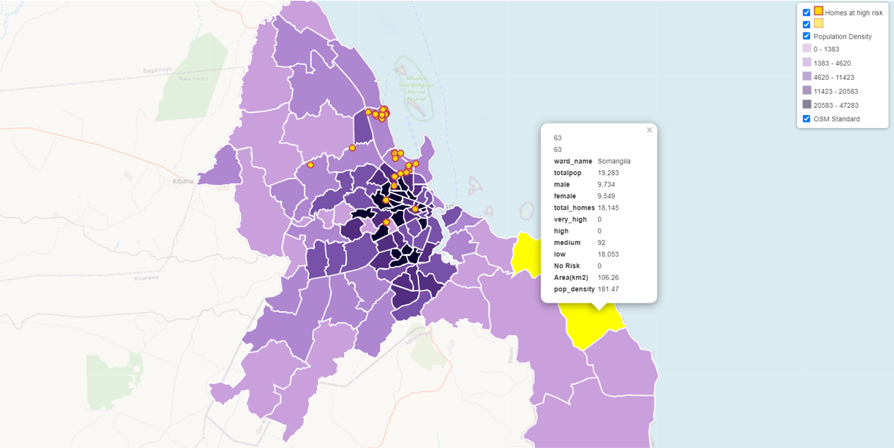 Figure 1. this is how its supposed to look! :(
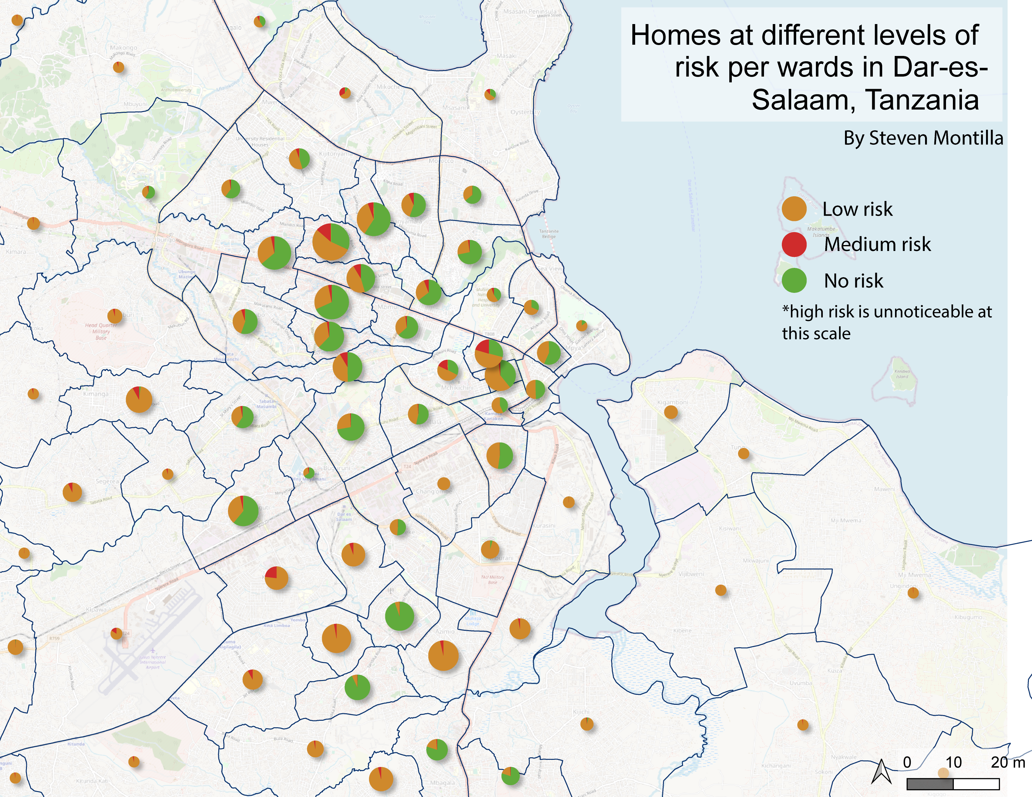 Figure 2. Risk levels of homes per ward
pie charts vary in size according to population density of the ward
Figure 2. Risk levels of homes per ward
pie charts vary in size according to population density of the ward
DATA SOURCES
Open Street Map: OpenStreetMap is a free, editable map of the whole world that is being built by volunteers largely from scratch and released with an open-content license. (About Open OpenStreetMap linked above)
- DATA: planet_osm_polygon: From OSM provided by Prof. Joe Holler. IMPORTANT: included attribute building:material
Resilience Academy: Resilience Academy is a partnership between four academic institutions in Tanzania: Ardhi University (ARU), University of Dar es Salaam (UDSM), Sokoine University of Agriculture (SUA) and State University of Zanzibar (SUZA) with the University of Turku (UTU) from Finland. It is an initiative of the Tanzania Urban Resilience Program (TURP), a partnership between the Government of Tanzania, the World Bank, and the Foreign, Commonwealth and Development Office (FCDO).(Resilience Academy website linked above) - DATA: - Dar es Salaam Administrative Wards - Dar Es Salaam Flood Scenarion 25-200cm - use in analysis: this information was used to score homes that intersected with the different flood scenarios with their respective risk score, and the administrative wards were used to aggregate the results and map our findings.
Acknowlegments
Thanks to Prof. Joe Holler for the help and putting the lab together and to Maddie Tango and Sanjana Roy for answering my questions and being willing to help!